This post aims to explain mathematically how populations change.
Our first attempt is based on ideas put forward by Thomas Malthus’ article “An Essay on the Principle of Population” published in 1798.
Let 

Assume in a small interval 
births =

deaths =

where 
It follows that the change of total population during time interval

where 
Dividing by 

which is
a first order differential equation.
Since (1) can be written as

integrate with respect to
leads to

where 
If at 

and so
The result of our first attempt shows that the behavior of the population depends on the sign of constant 


The world population has been on a upward trend ever since such data is collected (see “World Population by Year“)
Qualitatively, our model (2) with 
Therefore, it is doubtful that model (1) is The One.
Our second attempt makes a modification to (1). It takes the limitation factors into consideration by replacing constant 

where 

Replace

Since
Let 

This is the Logistic Differential Equation.
Written differently as
the Logistic Differential Equation is also a Bernoulli’s equation (see “Meeting Mr. Bernoulli“)
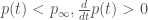
Let’s understand (5) geometrically without solving it.
Two constant functions, 


and

Plot 


Fig. 1
At point 


Similarly, at point 
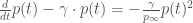
The model equation can also tell the manner in which
Let 


As an equation with unknown 

Therefore,


and


Consequently
where 
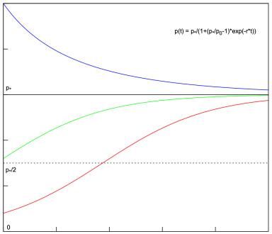
Fig. 2
If 


Next, let’s solve the initial-value problem analytically for
Instead of using the result from “Meeting Mr. Bernoulli“, we will start from scratch.
At 

Expressed in partial fraction,
Integrate it with respect to

gives

where
i.e.,

Since 

and so
Hence,

Solving for
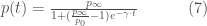
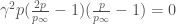
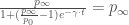
We proceed to show that (7) expresses the value of
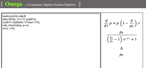
Fig. 3
From (7), we have

It validates Fig. 1.
(7) also indicates that none of the curves in Fig. 2 touch horizontal line 
If this is not the case, then there exists at least one instance of
It follows that
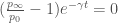
Since 

But this contradicts the fact that (7) is the solution of the initial-value problem (6) where 
Reflected in Fig.1 is that
Last, but not the least,

Hence the title of this post.